Plot fqpca loading functions with ggplot2

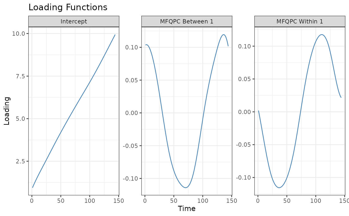
S3 method for class 'fqpca_object'. Given a fqpca object, plot the loading functions using ggplot2 facets.

Usage

# S3 method for class 'mfqpca_object'
plot(x, pve.between = 0.95, pve.within = 0.95, ...)

Arguments

x

An object output of the fqpca function.

pve.between

Percentage of explained variability to determine the number of components.

pve.within

Percentage of explained variability to determine the number of components.

...

Further arguments passed to or from other methods.

Value

A ggplot object plotting the intercept and FQPC curves.

Examples

n.individuals <- 20
n.repeated <- 10
n.time = 144
N <- n.repeated * n.individuals

group <- rep(1:n.individuals, each=n.repeated)

# Define score values using a normal distribution
c1.vals <- rnorm(n.individuals)
c1.vals <- c1.vals[match(group, unique(group))]
c2.vals <- rnorm(N)

# Define principal components
pcb <- sin(seq(0, 2*pi, length.out = n.time))
pcw <- cos(seq(0, 2*pi, length.out = n.time))

# Generate a data matrix and add missing observations
Y <- c1.vals * matrix(pcb, nrow = N, ncol=n.time, byrow = TRUE) +
c2.vals * matrix(pcw, nrow = N, ncol=n.time, byrow = TRUE) +
matrix(seq(1, 10, length.out=n.time), nrow = N, ncol=n.time, byrow = TRUE)
Y <- Y + matrix(rnorm(N*n.time, 0, 0.4), nrow = N)
Y[sample(N*n.time, as.integer(0.2*N))] <- NA

results <- mfqpca(
   data = Y, group=group, npc.between = 1, npc.within=1, quantile.value = 0.5,
   periodic=FALSE, seed=1)
plot(results)